MiLB Run-Expectancy Matrix
Overview
In this project, I converted Minor League play-by-play data into a run-expectancy matrix to determine the run values used in weighted on-base average (wOBA), weighted runs above average (wRAA) and weighted runs created plus (wRC+).
Introduction
I came into this summer with little experience coding in R but was determined to hone my skills in the language by completing an independent, hands-on baseball analytics project. At the same time, I interned in the front office of the Tacoma Rainiers, the Seattle Mariners’ Triple-A affiliate. Every day I combed through players’ pages on MiLB.com, looking for noteworthy metrics or trends in game-logs to include in the game notes and stat packs that I distributed to coaches and media members. Unfortunately, I was underwhelmed by the resources at my disposal. At the Major League level, there exists a seemingly infinite amount of data readily accessible for public consumption. On the other hand, advanced statistics at the Minor Leauge level are scarce. This makes it far harder for analysts to track player development, estimate a prospect’s trade value, project Major League performance and more.
Motivated by the lack of information, I decided to create and publish MiLB wOBA, wRAA and wRC+ statistics, along with a run-expectancy (RE24) matrix. Please note: this was a personal project and is not Tacoma Rainiers intellectual property done with the knowledge of Rainiers staff.
Data Collection
The MiLB play-by-play data used for the project is acquired through Bill Petti’s “baseballr” package. To obtain this data, I used the “lubridate” package to compile every game id for a given day. It is important to note that levels_id designates the given level of the play-by-play data. c(1) is the code for MLB data, c(11) for Triple-A, c(12) for Double-A, c(13) for High-A, c(15) for Low-A, c(5442) for Rookie Advanced, c(16) for Rookie ball, and c(17) for Winter League. I started this process on opening day, which for this case, was the Triple-A opening day on April 4. Then, I cycled through each day until the end of the season. However, here is where I encountered my first problem. Across Minor League baseball, Monday is a scheduled off day at all levels. Because of this, when the loop reached a date that was a Monday, it would stop running. To fix this, I implemented an if() statement that would skip the Monday date and move to Tuesday, where there are games. One limitation of this is that there are a small number of Monday games randomly placed throughout the schedule at any given Minor League level. By taking this approach, I omitted the run-expectancy data from these games. However, in the grand scheme of a season’s worth of data, the trade-off of leaving out a few games in order to make the code run effectively was worth it. The next step was pulling the pitch-by-pitch data for the given game id, and adding that to a data frame of the pitch-by-pitch data for all games on a given date. Then, I converted the pitch-by-pitch data into play-by-play data by eliminating all pitches from a given at-bat except for the final one. Finally, I added this synthesized play-by-play data to a data frame with all play-by-play data up to the date the loop is currently on.
# Set j as the date on which games start. In this case, it is set as
# Triple-A opening day
j <- as.Date("2022-04-05")# Creates play-by-play data frame
repeat {

  # Skips Monday (Monday's are MiLB off-days)
  if(weekdays.Date(j) == "Monday"){
    j <- j + 1
  }

  id <- mlb_game_pks(j, level_ids = c(11))
  game_id <- as.data.frame(id$game_pk)

  i <- 1
  for (i in 1:nrow(game_id)) {
    try( {

      # Resets the single_game_id variable for every different game
      single_game_id <- id$game_pk[i]

      # Gets play-by-play data for a single game on a single day
      single_game_data <- mlb_pbp(single_game_id)

      # Play-by-play data for an entire day
      single_day_pitch_data <- rbind(single_day_pitch_data, single_game_data, fill = TRUE)

      # Creates inning.description to delete pitch-by-pitch data, keeping only
      # one pitch per at-bat
      single_day_pitch_data$inning.description <- paste(single_day_pitch_data$about.inning, single_day_pitch_data$result.description)
      cleaned_day_plays <- distinct(single_day_pitch_data, inning.description, .keep_all = TRUE)

    }, TRUE
    )
  }

  # Goes to the next day
  j <- j + 1

  # Stops when the current date is reached
  if (j == "2022-10-01") {
    break
  }
}
Next, I indexed the complete play-by-play data in order to make the following computations easier.
indexed_plays <- subset(cleaned_day_plays, result.description != "TRUE")
indexed_plays$index_number <- row.names(indexed_plays)# Chronologically sorted play-by-play data
final_plays <- indexed_plays[order(as.numeric(indexed_plays$index_number), decreasing = TRUE), ]
Data Cleaning
While the play-by-play data is very detailed, at the Minor League level there are many variables that are not logged or are logged incorrectly. Because of this, an extensive data cleaning process is needed to convert the scraped play-by-play data into data that can be turned into a run-expectancy matrix. The first step was to add the score of the game before the game, so that the pre-play and post-play scores could be compared to determine how many runs were scored on the play. I did this using a simple for loop that set the pre-play score of a given play equal to the post-play score of the previous play, except for when the previous play occurs in a different game than the next play.
original_away_score <- rep(NA, nrow(final_plays))
original_home_score <- rep(NA, nrow(final_plays))# Creates accurate log of the score before each play
i <- 2
repeat{

  # Set the pre-play score equal to the post-play score of the previous play
  original_away_score[i] <- final_plays$result.awayScore[i-1]
  original_home_score[i] <- final_plays$result.homeScore[i-1]

  # If there is a new game, set both scores equal to zero
  if (isTRUE(final_plays$game_pk[i] != final_plays$game_pk[i - 1])){
    original_away_score[i] <- 0
    original_home_score[i] <- 0
  }

  # Stop the repeat when finished
  if (i == nrow(final_plays)){
    break
  }
  i <- i + 1
}# Update play-by-play data to include the score before every play
final_plays %>%
  mutate(details.awayScore = original_away_score,
         details.homeScore = original_home_score) -> final_plays
final_plays$details.awayScore[1] <-  0
final_plays$details.homeScore[1] <-  0
The scraped data includes where baserunners are after the play, but it does not indicate where the runners are before. Thus, the next step is replicating the process of the score with the baserunners. Note that this time the runners reset for both new games and new innings.
# Create necessary variables
matchup.preOnFirst.id <- rep(NA, nrow(final_plays))
matchup.preOnSecond.id <- rep(NA, nrow(final_plays))
matchup.preOnThird.id <- rep(NA, nrow(final_plays))
matchup.preOnFirst.name <- rep(NA, nrow(final_plays))
matchup.preOnSecond.name <- rep(NA, nrow(final_plays))
matchup.preOnThird.name <- rep(NA, nrow(final_plays))# Create log player names and ids before each play
i <- 2
repeat{

  # Set the pre-play names and ids equal to the names equal to the post-play
  # Names and ids of the previous play
  matchup.preOnFirst.id[i] <- final_plays$matchup.postOnFirst.id[i-1]
  matchup.preOnSecond.id[i] <- final_plays$matchup.postOnSecond.id[i-1]
  matchup.preOnThird.id[i] <- final_plays$matchup.postOnThird.id[i-1]
  matchup.preOnFirst.name[i] <- final_plays$matchup.postOnFirst.fullName[i-1]
  matchup.preOnSecond.name[i] <- final_plays$matchup.postOnSecond.fullName[i-1]
  matchup.preOnThird.name[i] <- final_plays$matchup.postOnThird.fullName[i-1]

  # If there is a new game, everything resets
  if (final_plays$game_pk[i] != final_plays$game_pk[i - 1]){
    matchup.preOnFirst.id[i] <- NA
    matchup.preOnSecond.id[i] <- NA
    matchup.preOnThird.id[i] <- NA
    matchup.preOnFirst.name[i] <- NA
    matchup.preOnSecond.name[i] <- NA
    matchup.preOnThird.name[i] <- NA
  }

  # If there is a new inning, everything resets
  if (final_plays$about.halfInning[i] != final_plays$about.halfInning[i - 1]){
    matchup.preOnFirst.id[i] <- NA
    matchup.preOnSecond.id[i] <- NA
    matchup.preOnThird.id[i] <- NA
    matchup.preOnFirst.name[i] <- NA
    matchup.preOnSecond.name[i] <- NA
    matchup.preOnThird.name[i] <- NA
  }

  # Stop the repeat when finished
  if (i == nrow(final_plays)){
    break
  }
  i <- i + 1
}# Update final plays data frame to include pre-play baserunners
final_plays %>%
  mutate(matchup.preOnFirst = matchup.preOnFirst.id,
         matchup.preOnSecond = matchup.preOnSecond.id,
         matchup.preOnThird = matchup.preOnThird.id,
         matchup.preOnFirst.name = matchup.preOnFirst.name,
         matchup.preOnSecond.name = matchup.preOnSecond.name,
         matchup.preOnThird.name = matchup.preOnThird.name) -> final_plays
Here is where I encountered my first serious issue with the way certain games were logged. For some reason, occasionally games would be input incorrectly and runners would appear on first base before they were up to bat in an inning. To fix this, if there was an instance in a game of a runner occurring on first during the at-bat when they were on-deck, the entire game was removed from the data set to ensure the accuracy of the overall data frame.
# There is an issue with the way some games are logged where the baserunners
# Are displayed out of chronological order. This deletes those games
i <- 1
repeat{
  if (isTRUE(final_plays$matchup.postOnFirst.id[i] == final_plays$matchup.batter.id[i + 1])) {
    final_plays <- final_plays %>%
      filter(game_pk != game_pk[i])
  }
  if (i == nrow(final_plays)){
    break
  }
  i <- i + 1
}
Runner Destinations
The next challenge I faced was determining the destination of the batter after a given play. This is necessary because a crucial part of the run-expectancy matrix is tracking runners throughout the play so one can compare the pre-play state (combination of runners on base and outs) with the post-play one.
bat_d <- rep(NA, nrow(final_plays))
run1_d <- rep(NA, nrow(final_plays))
run2_d <- rep(NA, nrow(final_plays))
run3_d <- rep(NA, nrow(final_plays))# Log batter destinations
for (i in 1:nrow(final_plays)) {

  # If the batter id equals the post-play id of a runner on a certain base,
  # The batter destination is that base
  if (isTRUE(final_plays$matchup.batter.id[i] == final_plays$matchup.postOnFirst.id[i])) {
    bat_d[i] <- 1}
  if (isTRUE(final_plays$matchup.batter.id[i] == final_plays$matchup.postOnSecond.id[i])) {
    bat_d[i] <- 2}
  if (isTRUE(final_plays$matchup.batter.id[i] == final_plays$matchup.postOnThird.id[i])) {
    bat_d[i] <- 3}

  # If the batter homers, their destination will be home
  if (isTRUE(grepl("homers", final_plays$result.description[i]))) {
    bat_d[i] <- 4
  }
}
However, as one can clearly see, this only tracks the batter destination. To find runner destinations, I had to first determine which runners scored on a given play, which I did by making a separate data frame that contained the play description of each play, split by sentence.
scoring <- str_split(final_plays$result.description, ".   ", simplify = TRUE)
scoring <- sub("[0-9.]+$", "", scoring)
Next, I went through each sentence, looking for instances of the word “scoring,” as this obviously indicates plays in which a runner scores. If the sentence did not have “scores,” I removed it from the data frame. If it did, I removed everything in the sentence except for the player’s name who scored. One limitation of this process is that it takes a very long time to run. I am currently working on an alternative method without using for loops, but until then, if one runs this code, they should do so overnight.
i <- 1
repeat {
  for (j in 1:ncol(scoring)){

    # Get rid of plays in which no one scores
    if (isFALSE(grepl("scores", scoring[i, j]))){
      scoring[i, j] <-  NA
    }

    # If it is a scoring play, delete everything except for the player's name
    if (isTRUE(grepl("scores", scoring[i, j]))){
      scoring[i, j] <- gsub(" scores", "", scoring[i, j])
      scoring[i, j] <- gsub("scores", "", scoring[i, j])
    }
  }

  # Delete unnecessary space
  scoring <- gsub(" ", "", scoring)
  if (i == nrow(scoring)){
    break
  }
  i <- i + 1
}
# Delete unnecessary spaces
scoring <- gsub(" ", "", scoring)
Once I knew who scored as a result of each play, I could determine the post-play destinations of each of the baserunners for every play. I did this by comparing the pre-play baserunners with the post-play baserunners and scoring matrix. For example, if a runner was on first before the play, if they remained on-base after the play, that base would be their play destination. If they were not on-base after the play, but they did score, then their destination would be home.
# Create final destination for runner on first
for (i in 1:nrow(final_plays)) {

  # If the runner on first id equals the post-play id of a runner on a certain base,
  # The runner destination is that base
  if (isTRUE(final_plays$matchup.preOnFirst[i] == final_plays$matchup.postOnFirst.id[i])) {
    run1_d[i] <- 1}
  if (isTRUE(final_plays$matchup.preOnFirst[i] == final_plays$matchup.postOnSecond.id[i])) {
    run1_d[i] <- 2}
  if (isTRUE(final_plays$matchup.preOnFirst[i] == final_plays$matchup.postOnThird.id[i])) {
    run1_d[i] <- 3}

  # If the runner on first scores, their destination will be home
  for (j in 1:ncol(scoring)) {
    if (isTRUE(final_plays$matchup.preOnFirst.name[i] == scoring[i, j])){
      run1_d[i] <- 4
    }
  }
}# Create final destination for runner on second
for (i in 1:nrow(final_plays)) {

  # If the runner on second id equals the post-play id of a runner on a certain base,
  # The runner destination is that base
  if (isTRUE(final_plays$matchup.preOnSecond[i] == final_plays$matchup.postOnSecond.id[i])) {
    run2_d[i] <- 2}
  if (isTRUE(final_plays$matchup.preOnSecond[i] == final_plays$matchup.postOnThird.id[i])) {
    run2_d[i] <- 3}

  # If the runner on second scores, their destination will be home
  for (j in 1:ncol(scoring)) {
    if (isTRUE(final_plays$matchup.preOnSecond.name[i] == scoring[i, j])){
      run2_d[i] <- 4
    }
  }
}# Create final destination for runner on third
for (i in 1:nrow(final_plays)) {

  # If the runner on second id equals the post-play id of a runner on a certain base,
  # The runner destination is that base
  if (isTRUE(final_plays$matchup.preOnThird[i] == final_plays$matchup.postOnThird.id[i])) {
    run3_d[i] <- 3}

  # If the runner on third scores, their destination will be home
  for (j in 1:ncol(scoring)) {
    if (isTRUE(final_plays$matchup.preOnThird.name[i] == scoring[i, j])){
      run3_d[i] <- 4
    }
  }
}# Add batter and baserunner destination to plays data frame
final_plays %>%
  mutate(bat_dest = bat_d, run1_dest = run1_d, run2_dest = run2_d,
         run3_dest = run3_d) -> final_plays
Creating the Run-Expectancy Matrix
First, I created a new data frame for the purpose of creating the run-expectancy matrix. I did this for two reasons. The first is that if I wanted to use the cleaned final_plays data frame for other projects, I would not want any of the alterations that I made to the data in the creation of the run-expectancy matrix. The second is that there was a significant amount of trial and error involved in the creation of the final matrix, and rather than have to redo the entire cleaning process of the final_plays data every time I encountered an error in the run-expectancy matrix, it was far easier to start fresh each time.
# Create necessary data frames
re24_plays <- data_frame()
RUNS_1 <- data_frame()
re24_plays <- final_plays# Set all NAs equal to 0, allows following code to run correctly
re24_plays[is.na(re24_plays)] <- 0
Next, I had to perform basic data preparation for later calculations. This included the creation of a runs, runs scored, and outs on play variables, which are self-descriptive. The other is a half inning variable, that I created by combining the game identification number, the inning number, and the half inning (top or bottom), to make a unique tag for every half-inning of every game in a season.
# Creates essential variables for the calculation of run-expectancy
re24_plays %>%
  mutate(
    # RUNS equals the total number of runs in the game
    RUNS = details.homeScore + details.awayScore,

    # Create HALF.INNING so that the plays can be grouped by half inning
    # later
    HALF.INNING = paste(game_pk, about.inning, about.halfInning),

    # OUTS.ON.PLAY is the number of outs recorded on the play
    OUTS.ON.PLAY = count.outs.end - count.outs.start,

    # Create RUNS.SCORED variable to track runs scored every play
    RUNS.SCORED =
      (bat_dest > 3) + (run1_dest > 3) +
      (run2_dest > 3) + (run3_dest > 3)) -> re24_plays
I created the unique half-inning tag so that I could determine the maximum runs scored in a given half-inning. This is significant in the calculation of run-expectancy because it allowed me to ascertain how many more runs would score after a given event, thus giving the individual run-expectancy of that event. I did this using “RUNS.ROI,” which represents the difference between the total runs scored in a half-inning and the number of runs that had been scored up to the point of the play at which the run-expectancy was being calculated.
# Group by half inning (run expectancy matrices look at each half inning as
# independent events)
re24_plays %>%
group_by(HALF.INNING) %>%
# Create crucial variables in the creation of the matrix
summarize(Outs.Inning = sum(OUTS.ON.PLAY),
Runs.Inning = sum(RUNS.SCORED),
Runs.Start = first(RUNS),
MAX.RUNS = Runs.Inning + Runs.Start) -> half_innings
# Add half innings groups back to main data frame
# RUNS.ROI is the difference between the maximum runs scored in the inning
# and the number of runs that have already been scored
re24_plays %>%
inner_join(half_innings, by = "HALF.INNING") %>%
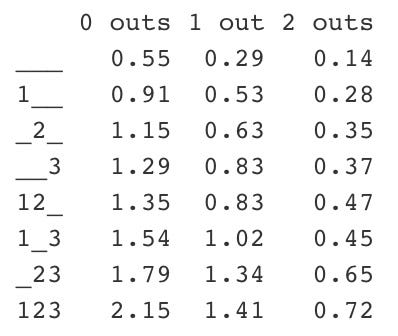
mutate(RUNS.ROI = abs(MAX.RUNS - RUNS)) -> re24_playsOnce I had the necessary run and inning information, I could label each pre-play and post-play situation by the number of outs and people on base. This is called the “state” of the play. For example, if there are runners on first and third with one out before the play, the state will be “1_3 1.” If the play that occurs is a sacrifice fly, the runner on third will score and the runner on first will stay there, giving a “new state” of “1__ 2.” I created this new state by evaluating the runner destination for each person on base, as well as the batter.
# Creates the state (or situation) prior to the play
re24_plays %>%

  # BASES represents which runners are currently on which base
  mutate(BASES =
           paste(ifelse(matchup.preOnFirst > 0, 1, 0),
                 ifelse(matchup.preOnSecond > 0, 1, 0),
                 ifelse(matchup.preOnThird > 0, 1, 0), sep = ""),

         # STATE adds the number of outs to BASES
         STATE = paste(BASES, count.outs.start)) -> re24_plays# Create the state (or situation) following  the play
re24_plays %>%

  # Find which runners end up where
  mutate(NRUNNER1 =
           as.numeric(run1_dest == 1 | bat_dest == 1),
         NRUNNER2 =
           as.numeric(run1_dest == 2 | run2_dest == 2 |
                        bat_dest == 2),
         NRUNNER3 =
           as.numeric(run1_dest == 3 | run2_dest == 3 |
                        run3_dest == 3 | bat_dest == 3),

         # Find the resulting outs on the play
         NOUTS = count.outs.start + OUTS.ON.PLAY,

         # Create new bases and state variables to reflect the results of the play
         NEW.BASES = paste(NRUNNER1, NRUNNER2,
                           NRUNNER3, sep = ""),
         NEW.STATE = paste(NEW.BASES, NOUTS)) -> re24_plays
Finally, before calculating run-expectancy, I had to do a final round of data cleaning. The first step was removing plays with the same state in which no runs scored, as these were likely incorrectly logged and thus would affect the accuracy of the run-expectancy matrix. The second step was removing half-innings in which less than three outs were recorded, as these are innings ended by walk-offs. I did this because in these instances a team is playing to win the game, rather than to maximize their runs as they would in all other situations, so walk-off half-innings would not accurately reflect true run-expectancy.
# Filter out plays that have the same state with no runs scored
re24_plays %>%
  filter((STATE != NEW.STATE) | (RUNS.SCORED > 0)) -> re24_plays# Filter out innings that end with less than three outs
re24_plays %>%
  filter(Outs.Inning == 3) -> re24_plays_final
Once all the necessary steps were completed, I was ready to calculate the run-expectancy matrix. I did this by determining the average run-expectancy for each state, then combining them into one easy to read matrix.
# Final calculations for run-expectancy matrix
re24_plays_final %>%
  group_by(STATE) %>%

  # Each state recieves its corresponding run expectancy
  summarize(Mean = mean(RUNS.ROI)) %>%
  mutate(Outs = substr(STATE, 5, 5)) %>%
  arrange(Outs) -> RUNS_1# Create run expectancy matrix
re24 <- matrix(round(RUNS_1$Mean, 2), 8, 3)# Give matrix appropriate row and column names
dimnames(re24)[[2]] <- c("0 outs", "1 out", "2 outs")
dimnames(re24)[[1]] <- c("___", "__3", "_2_", "_23",
                         "1__", "1_3", "12_", "123")
Creating Run Values
The next step was calculating the run values for each batted ball event. A run value is the increase in expected runs scored by the batting team after a given batted ball event. For example, if teams always score 1 run because of or after a single, the un-scaled run value of a single will simply be 1. To do this, I first had to determine the individual run values of each play.
# Preparation work for finding run values
re24_plays %>%

  # Concentrate run values by state
  left_join(select(RUNS_1, -Outs), by = "STATE") %>%
  rename(Runs.State = Mean) %>%
  left_join(select(RUNS_1, -Outs),
            by = c("NEW.STATE" = "STATE")) %>%
  rename(Runs.New.State = Mean) %>%
  replace_na(list(Runs.New.State = 0)) %>%

  # Find run value of each play
  mutate(run_value = Runs.New.State - Runs.State +
           RUNS.SCORED) -> re24_plays
Then I calculated the run value of an out by determining the average run value correlated with each out. As you can see, the run value of an out is negative, which makes perfect logical sense.
# Create necessary variable
outs <- rep(0, nrow(re24_plays))# Find plays that resulted in outs
re24_plays %>%
  filter(OUTS.ON.PLAY > 0) -> outs# Find run value of outs
outs %>%
  summarize(mean_run_value = mean(run_value)) -> mean_outs
Next, I calculated the mean run values of each way of getting on base (1B, 2B, 3B, HR, BB and HBP), other than reaching on an error. The process for each of these was identical, and here is an example of how I calculated the run value of a single. Note the line of code where the un-scaled single run value is subtracted by the run value of an out to “scale” it. This is necessary because we are not interested in how many runs a way of getting on base generates, we are interested in how many more runs that way of getting on base generates compared to an out. Using the example of a single from before, if the un-scaled run value of a single is 1, and the run value of an out is -.25, the true, or “scaled,” run value of a single would be 1.25.
# Create necessary variable
single <- rep(0, nrow(re24_plays))# Find all instances of a single
for (i in 1:nrow(re24_plays)){
  if (isTRUE(grepl("singles", re24_plays$result.description[i]))) {
    single[i] <- 1
  }
}# Select plays with a single
re24_plays %>%
  mutate(singles = single) %>%
  filter(singles == 1) -> singles# Find run value of singles by finding the mean run values of all plays with
# a single
singles %>%
  summarize(mean_run_value = mean(run_value)) -> mean_singles# Find the run value of a single to that of an out
SINGLE <- mean_singles - mean_outs
Calculating Linear Weights
In order to determine the linear weights that are used in the calculation of wOBA, the league average wOBA must first be scaled so that it is equal to league average OBP, which can be done with the play-by-play data. To do this, I first had to find all instances of sacrifice flies and intentional walks in the data.
# Create necessary variable
sf <- rep(0, nrow(re24_plays))
ibb <- rep(0, nrow(re24_plays))# Find all instances of a sacrifice fly
for (i in 1:nrow(re24_plays)){
  if (isTRUE(grepl("sacrifice fly", re24_plays$result.description[i]))) {
    sf[i] <- 1
  }
  if (isTRUE(grepl("intentionally walks", re24_plays$result.description[i]))) {
    ibb[i] <- 1
  }
}# Select plays with a sacrifice fly
re24_plays %>%
  mutate(sf = sf, ibb = ibb) -> re24_plays
Once I had these values, I could then calculate the “wOBA Multiplier,” which is the un-scaled league wOBA, as well as the league OBP.
# Create "wOBA Multiplier" by calculating the league wOBA figure
woba_multiplier <-
  (HBP*nrow(hbp) + BB*nrow(walks) + SINGLE*nrow(singles) + DOUBLE*nrow(doubles)
   + TRIPLE*nrow(triples) + HR*nrow(home_runs))/(nrow(re24_plays) - sum(ibb) - sum(sf))# Calculate the league OBP figure
league_obp <-
  (nrow(hbp) + nrow(walks) + nrow(singles) + nrow(doubles) + nrow(triples)
   + nrow(home_runs))/(nrow(re24_plays) - sum(ibb))
Next, I calculated the wOBA Scale by dividing the league OBP by the wOBA multiplier. I then multiplied the wOBA scale by the run values so that the league wOBA is equal to the league OBP.
woba_scale <- league_obp / woba_multiplier# Multiply the play run values by the wOBA scale to obtain the weights used in
# the wOBA calculation
woba_weights <- c(woba_scale*HBP, woba_scale*BB, woba_scale*SINGLE,
                  woba_scale*DOUBLE, woba_scale*TRIPLE, woba_scale*HR)
After correctly scaling the weights, I finished the project by creating a simple data table that displayed the weights.
# Create an easily readable table containing the wOBA weights
linear_weights_table <- as.data.frame(woba_weights)# Ensure the table is named correctly
rownames(linear_weights_table) <- c("HBP", "BB", "1B", "2B", "3B", "HR")
colnames(linear_weights_table) <- c("Weights")
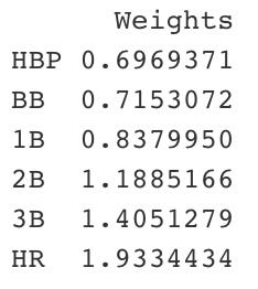
LINEAR WEIGHTS TABLE
From here, one can use the weights to calculate a player’s individual wOBA, wRAA, and wRC+ metrics. This is valuable as these statistics are far more valuable in evaluating prospects than the conventional batting average, on-base percentage, and slugging percentage.
Another potential issue is the influence of park factors in the wRC+ calculations. Park factors are included as a way of attempting to eliminate the impact of a batter playing at a “hitters park” or “pitchers park.” However, there were extreme disparities in Minor League park factors due to the wide variety in stadiums and conditions. For example, to hit a home run to center field at Cheney Stadium (home of the Triple-A Tacoma Rainiers) a batter must clear the 29-foot batters’ eye that lies 425 feet from home plate. The issue with this is that they have a much greater effect on wRC+ numbers than at the Major League level because a player may not play all their games at the given level. Hypothetically, if a player in Double-A got called up to Triple-A for a month or so and played incredibly well with the majority of their games coming on the road in high run scoring environments. If the park factor of their home stadium is below 1, then even though they played a disproportionate number of games on the road, their numbers would be artificially inflated.
In the future, I hope to apply these weights to batted ball data to create xwOBA. Unfortunately, only a limited number of Minor League stadiums have the necessary equipment to effectively measure batted ball data. However, every Triple-A Pacific Coast League stadium can record batted ball data, so perhaps my project would be limited to this league only. This would still be valuable, as given the difficulty of projecting success of Minor League prospects, the more information accessible to teams and the public, the better.

